Best practices in data cleaning and preparation process

Almost every statistical work on collected data starts with data exploration and visual assessment of its layout. It gives a really fast initial overview of data distribution, in addition to recognizing the nature of the phenomenon being studied. Furthermore, it helps us decide whether to subject the data to some operations before performing statistical analyses or not. Why is good to have best practices in the data cleaning and preparation process? Because expensive data are worth it. Inferences are drawn well only in the circumstances where we established regularity and smoothness of gathered data. Of course, there are statistical techniques that do not require such preparation (e.g. natural networks, support vector machines), but getting to know data is good analytical practice. Below, we put some basic visual methods and examples of what to do with data that shows some irregularities.

Visual exploration methods

The first-line in data exploration is visual techniques which are related to assessment of: 

  1. Histograms – which shows general shape of single variable distribution. After variable standardization, histogram detects outliers defined as a certain observations located outside a laid down value interval, expressed in units of standard deviation. Usually, such an interval contains values lying between -3SD and 3SD. 
  2. Boxplots – which also shows a shape of single variable distribution but in a slightly different way. Contrary to histogram, we will not see here the degree to which variable scores cluster around extreme or central values of distribution. But instead of it, we can observe data quartiles (including the median), which are a different type of information about variable distribution. Outliers located outside the whiskers are defined as observations that are out of the interquartile range*1.5.
  3. Scatterplots – which shows relation between two variables. In these case, outlier is an observation that are the most distant from the regression line (line or curve in the context of non-linear model) and doesn’t follow the general pattern. We can detect them “by eye” or using a formal criterion based on Cook’s Distance.

*More formal way to detect outliers are statistical tests such as: Grubbs’s test, Dixon’s test and Rosner’s test (which are provided for example by `outliers` R package dedicated to data exploration).

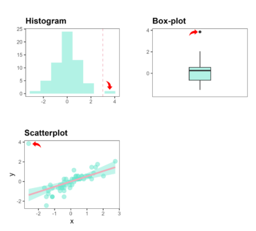
Typical outlier charts

The charts presented below are very practical in data exploration process and show three methods of detecting outliers

detecting outliers in preprocessing exploration data step histogram, scatterplot, boxplot

So, what can we do to improve the quality of our data, and consequently get more reliable statistical analysis results? 

Detection of outliers and what next?

One of the most commonly used method in data exploration step is removing outliers and replacing them by mean or median value. Good information is that you can do that „trick” with only an Excel at your disposal. 

Certainly more advanced (if not the most) statistical method of data imputation is provided by `missForest` R package. This method is based on Random Forest algorithm, which impute not only continuous data, but also these categorical ones. It works on complex data, based on the entire dataset, takes into account nonlinear relations between variables and their interactions. This procedure is very useful and “safe” in data exploration phase. 

*It is assumed that number of `missings` should be less than 5%.

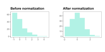
And the last one method - used when variable doesn’t follow a normal distribution is `normalization` provided by `bestNormalize` R package. Normal distribution is required when we use parametric statistical analysis (e.g. regression analysis, anova, t-test). This statistical assumption is not critical, but  sometimes is easy to be established, and improves estimates of statistical significance. 

The chart presented below shows how normalization works.

normalization of distribution